Creating a Map of the wine AOCs of France with geopandas and shapely

Important note: The code displayed in this notebook takes some time to execute (in my computer, about 10 minutes). To render the sphinx file, I had to modify the conf.py file and add: nb_execution_timeout = 1000 (defaults to 30).

In this post, I will be creating a map of the wine regions (AOC) of the Loire Valley, from open Data.

We will get the data from the open data source, do some simple transformations using shapely, and plot the result. We will also upload the result to Kaggle, so others can use our new data set.

Step 1: Download the dataset.

We will be getting the dataset from the French Government Open Data portal.

We download the .zip file, unzip it and place the shapefiles in a folder. In my case, here is the path to the shapefile:

path_to_shp = "aoc_map_20230605/2023-07-03_delim-parcellaire-aoc-shp.shp"

Now, we can import our libraries for the project:

import geopandas as gpd
import pandas as pd
from matplotlib import pyplot as plt

Step 2: Creating a GeoPandas GeoDataFrame

GeoPandas knows shapefiles, so this as simple as reading the file:

aoc_raw_data = gpd.read_file(path_to_shp)

aoc_raw_data.head(3)

	dt	type_prod	categorie	type_denom	signe	id_app	app	id_denom	denom	insee	cvi	nomcom	insee2011	nomcom2011	id_aire	crinao	grp_name1	grp_name2	geometry
0	Angers	NaN	Vin mousseux, Vin primeur, Vin tranquille	appellation	AOC	76	Anjou	173	Anjou	49001	1B200, 1B200M 1, 1R200S, 1R203S, 1R203S01, 1S2...	BRISSAC LOIRE AUBANCE	49001	LES ALLEUDS	133	NaN	NaN	NaN	MULTIPOLYGON (((440405.700 6696103.480, 440524...
1	Angers	NaN	Vin mousseux, Vin primeur, Vin tranquille	appellation	AOC	76	Anjou	173	Anjou	49002	1B200, 1B200M 1, 1R200S, 1R203S, 1R203S01, 1S2...	ALLONNES	49002	ALLONNES	133	NaN	NaN	NaN	MULTIPOLYGON (((476099.070 6692210.880, 476039...
2	Angers	NaN	Vin mousseux, Vin primeur, Vin tranquille	appellation	AOC	76	Anjou	173	Anjou	49003	1B200, 1B200M 1, 1R200S, 1R203S, 1R203S01, 1S2...	TUFFALUN	49003	AMBILLOU-CHATEAU	133	NaN	NaN	NaN	MULTIPOLYGON (((445501.950 6686844.110, 445500...

Our DataFrame has many different informations. Since this is from the French administration, all refers to French. Here are some of the relevant columns

• dt: Délégation territoriale This an administrative department. Not relevant as a wine origin division, but they cover kind of homogeneous areas. We are keeping this for our GeoDataFrame, at least to split it in the beginning and do some explorations.

• categorie: wine type(s)

• signe: it is always AOC.

• id_app: unique identifier for the AOC

• app: short for appellation, it is the name of the AOC.

• geometry: holds the geometry of the viticultural area parcels as Multipolygons.

Let’s see how many distinct administrative departments (dt) we have (note that I use the .size() command, this counts the number of rows. The granularity here is: towns x AOC name, so the number is not really relevant nor useful. This command is really just to have an idea on how we can start splitting the DataSet to explore it, because it is big).

# Get the distinct dt of the dataset
dt_distinct = aoc_raw_data.groupby("dt").size().reset_index(name="number_of_dt")
dt_distinct

	dt	number_of_dt
0	Angers	1380
1	Avignon	456
2	Bordeaux	2348
3	Colmar	356
4	Corse	270
5	Dijon	3004
6	Gaillac	263
7	La Valette du Var	184
8	Montpellier	707
9	Mâcon	1077
10	Narbonne	791
11	Pau	260
12	Tours	537
13	Valence	197

aoc_raw_data.head(2)

	dt	type_prod	categorie	type_denom	signe	id_app	app	id_denom	denom	insee	cvi	nomcom	insee2011	nomcom2011	id_aire	crinao	grp_name1	grp_name2	geometry
0	Angers	NaN	Vin mousseux, Vin primeur, Vin tranquille	appellation	AOC	76	Anjou	173	Anjou	49001	1B200, 1B200M 1, 1R200S, 1R203S, 1R203S01, 1S2...	BRISSAC LOIRE AUBANCE	49001	LES ALLEUDS	133	NaN	NaN	NaN	MULTIPOLYGON (((440405.700 6696103.480, 440524...
1	Angers	NaN	Vin mousseux, Vin primeur, Vin tranquille	appellation	AOC	76	Anjou	173	Anjou	49002	1B200, 1B200M 1, 1R200S, 1R203S, 1R203S01, 1S2...	ALLONNES	49002	ALLONNES	133	NaN	NaN	NaN	MULTIPOLYGON (((476099.070 6692210.880, 476039...

Step 3: Simplyfy Geometries

In order to make the treatment a bit less heavy, I simplify the geometry of the DataFame:

• I create a new DataFrame, simplified_data, with the same columns as aoc_raw_data. Then, I iterate over the rows of aoc_raw_data to add each row, with simplified geometry, to the new DataFrame

• I use gpd.simplify(). This is used to reduce the number of points in the polygon (which obviously reduces the size of it). I set the tolerance to 0.1, because we do not need a lot of precision for our DataSet, we are not going to use it for legal purpose. We are more interested in having something a bit lighter.

• I also use gpd.buffer()

• Both gpd.simplify() and gpd.buffer() are geoSeries, this is why we itrerate on each row of ````aoc_raw_data```

• The expression .to_frame().transpose() allows us to make a Series become a DataFrame, and then transpose it to insert it as a row in the simplified_data DataFrame.

# Set the tolerance value for simplification

tolerance = 0.1

# Create a new GeoDataFrame for simplified geometries
simplified_data = gpd.GeoDataFrame(columns=aoc_raw_data.columns)

# Iterate over each row in the original GeoDataFrame
for _, row in aoc_raw_data.iterrows():
    # Simplify the geometry of the current row
    simplified_geometry = row["geometry"].simplify(tolerance)

    # Buffer the simplified geometry to merge nearby polygons within the same MultiPolygon
    buffered_geometry = simplified_geometry.buffer(0)

    # Create a new row with the simplified and buffered geometry
    simplified_row = row.copy()
    simplified_row["geometry"] = buffered_geometry

    # Append the simplified row to the new GeoDataFrame
    simplified_data = pd.concat(
        [simplified_data, simplified_row.to_frame().transpose()], ignore_index=True
    )

# Convert the geometry column to the appropriate geometry type
simplified_data["geometry"] = gpd.GeoSeries(simplified_data["geometry"])

simplified_data.head(2)

	dt	type_prod	categorie	type_denom	signe	id_app	app	id_denom	denom	insee	cvi	nomcom	insee2011	nomcom2011	id_aire	crinao	grp_name1	grp_name2	geometry
0	Angers	NaN	Vin mousseux, Vin primeur, Vin tranquille	appellation	AOC	76	Anjou	173	Anjou	49001	1B200, 1B200M 1, 1R200S, 1R203S, 1R203S01, 1S2...	BRISSAC LOIRE AUBANCE	49001	LES ALLEUDS	133	NaN	NaN	NaN	MULTIPOLYGON (((442300.200 6697404.860, 442633...
1	Angers	NaN	Vin mousseux, Vin primeur, Vin tranquille	appellation	AOC	76	Anjou	173	Anjou	49002	1B200, 1B200M 1, 1R200S, 1R203S, 1R203S01, 1S2...	ALLONNES	49002	ALLONNES	133	NaN	NaN	NaN	MULTIPOLYGON (((476247.180 6692521.190, 476236...

Step 4: Dissolve the dataframe

Disolving the DataFrame takes A LOT of time.

But we will be happy to have a less heavy file at the end of all this process!

The shapely function unary_union allows us to dissolve the geometries of the GeoDataFrame, grouping them by a certain attribute.

To minimize the data and the execution time, we create a minimal DataFrame only_aoc by only keeping some columns from simplified_data.

from shapely.ops import unary_union

only_aoc = simplified_data[["app", "id_app", "dt", "geometry"]]

# Group the GeoDataFrame by the 'app' attribute
grouped_data = only_aoc.groupby(["app", "id_app"])

# Perform unary union within each group
merged_geometries = grouped_data["geometry"].apply(unary_union)

# Create a new GeoDataFrame with the merged geometries
aoc_data = gpd.GeoDataFrame({"geometry": merged_geometries}, crs=only_aoc.crs)

# Add the 'app' and 'id_app' attributes from the first row of each group
aoc_data["app"] = grouped_data["app"].first().values
aoc_data["id_app"] = grouped_data["id_app"].first().values
aoc_data["dt"] = grouped_data["dt"].first().values

Next, we reset the index to have all the information in rows. We also set the crs to EPSG:2154. This is the code for Lambert 93 projections, used in general in France (and specified in the shapefiles folders).

# Reset the index
aoc_data = aoc_data.reset_index(drop=True)

# Set the CRS:
aoc_data.crs = "EPSG:2154"

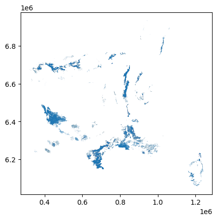
And then we save the data and we make a quick plot to see how it all looks. By the way, by “quick”, I mean “not quick at all”, the amount of data is important.

aoc_data.head(3)

	geometry	app	id_app	dt
0	MULTIPOLYGON (((1163696.340 6132355.130, 11636...	Ajaccio	291	Corse
1	MULTIPOLYGON (((841102.787 6663422.737, 841097...	Aloxe-Corton	126	Dijon
2	POLYGON ((1028787.850 6840673.780, 1028785.610...	Alsace grand cru Altenberg de Bergbieten	1187	Colmar

Step 5: Save the DataFrame

aoc_data.to_file('aoc.gpkg', driver='GPKG', layer='aocs_france')  

aoc_data.plot()  # I do this to see how it looks like, not a good plot -- by the way, it takes long

<Axes: >

Step 6: Plotting a Region: Loire Valley wines

Due to very heavy size of the DataFrame, we are going to only plot a part of it. We will take the “dt” of Angers (which is the west of the Loire Valley)

It is important to convert the CRS to 3857, it is one of the supported formats for Open Street Maps.

aoc_data_angers = aoc_data[aoc_data["dt"] == "Angers"]

aoc_data_angers = aoc_data_angers.to_crs("EPSG:3857")  # 2154 is unsupported, on

import contextily as ctx
import tilemapbase

tilemapbase.start_logging()
tilemapbase.init(create=True)
extent = tilemapbase.extent_from_frame(aoc_data_angers, buffer=5)

fig, ax = plt.subplots(figsize=(10, 10))

plotter = tilemapbase.Plotter(extent, tilemapbase.tiles.build_OSM(), width=1000)

plotter.plot(ax)

aoc_data_angers.plot(column="app", ax=ax, legend=False)

<Axes: >

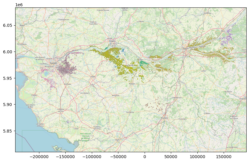
And then we save the map. Nottice the dpi parameter, it means: “dots per inch”, I use it to increase the quality of the image

ax.figure.savefig("./wines_loire.png", bbox_inches="tight", dpi=300)

Step 7: Making a folium map

Folium lets us do interactive maps for a website, an application or a notebook report. it is pretty neeat, but it can be ressource intensive. The last thing we want is a 100 MB webpage, so I will plot the data for the dt of Pau.

The newest versions of GeoPandas let you create a folium map directly with the .explore() method, which is AWESOME.

aoc_data_pau = aoc_data[aoc_data["dt"] == "Pau"]

import folium
#Use chatgpt to get the coordinates of places :)
m = folium.Map(location=[43.296482, -0.370027], zoom_start=8)

aoc_data_pau.explore(column="app", m=m, cmap="Dark2")

Make this Notebook Trusted to load map: File -> Trust Notebook

That’s it for today! I will be doing more with this, so bookmark this blog!

You can fin the dataset on this link on kaggle.

Writing my personal blog with sphinx and Jupyter Notebooks: Throwing some light to the motivations.   Get wine harvest data by French Region from a pdf